Data Wrangling & Preprocessing
Data wrangling is the process of cleaning raw data into analysis-ready format. Handle missing values (impute or drop), fix data types, remove duplicates, detect outliers (IQR or Z-score), and reshape data (melt/pivot). pandas is your primary tool. Expect to spend 60-80% of project time here.
Explain Like I'm 12
Imagine you just got a giant box of LEGO pieces, but they're all mixed up, some are broken, and some aren't even LEGO. Before you can build anything cool, you need to: sort them (data types), throw away broken ones (remove bad data), find missing pieces (handle nulls), and organize by color and size (reshape). That's data wrangling — getting your data ready before the fun part starts.
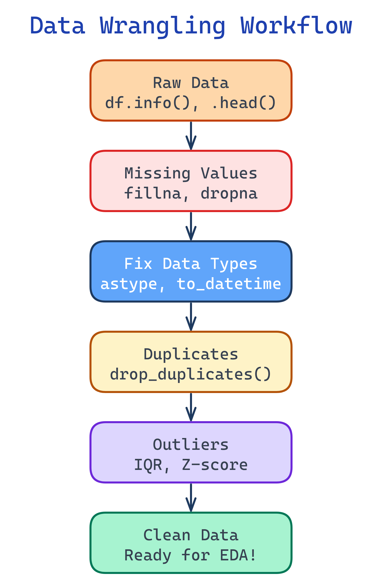
The Wrangling Workflow
Data wrangling follows a predictable pattern. Start by understanding what you have, then fix issues systematically.
Step 1: Inspect Your Data
Before fixing anything, understand what you're working with. These five commands tell you almost everything you need to know.
import pandas as pd

df = pd.read_csv('dataset.csv')

# Shape: how many rows and columns?
print(df.shape)              # (10000, 15)

# Column types and null counts
print(df.info())

# Statistical summary of numeric columns
print(df.describe())

# First few rows
print(df.head())

# Unique values per column (spot unexpected categories)
for col in df.select_dtypes(include='object'):
print(f"{col}: {df[col].nunique()} unique — {df[col].unique()[:5]}")df.info() first every time. It shows data types and null counts in one view. If a column that should be numeric shows as object, you have dirty values in it (like "$" or "N/A" strings).Step 2: Handle Missing Values
Missing data is the most common issue. Your strategy depends on how much is missing and why it's missing.
| Strategy | When to Use | Code |
|---|---|---|
| Drop rows | <5% missing, random | df.dropna(subset=['col']) |
| Drop column | >50% missing | df.drop('col', axis=1) |
| Fill with median | Numeric, has outliers | df['col'].fillna(df['col'].median()) |
| Fill with mean | Numeric, normal distribution | df['col'].fillna(df['col'].mean()) |
| Fill with mode | Categorical | df['col'].fillna(df['col'].mode()[0]) |
| Forward fill | Time series | df['col'].ffill() |
| Flag + fill | Missingness is informative | Create col_was_missing boolean column |
# Visualize missing data patterns
missing_pct = (df.isnull().sum() / len(df) * 100).sort_values(ascending=False)
print(missing_pct[missing_pct > 0])

# Strategy: create a "was_missing" flag, then impute
df['income_missing'] = df['income'].isnull().astype(int)
df['income'].fillna(df['income'].median(), inplace=True)

# For categorical columns, fill with the mode
df['city'].fillna(df['city'].mode()[0], inplace=True)

# For time series, use forward fill
df['temperature'].ffill(inplace=True)Step 3: Fix Data Types
Wrong types silently break calculations. A "price" column stored as a string can't be summed or averaged.
# String prices → numeric (remove $, commas)
df['price'] = df['price'].str.replace('[$,]', '', regex=True).astype(float)

# String dates → datetime
df['date'] = pd.to_datetime(df['date'], format='%Y-%m-%d')

# Categories with few unique values → category type (saves memory)
df['status'] = df['status'].astype('category')

# Boolean strings → actual booleans
df['is_active'] = df['is_active'].map({'yes': True, 'no': False, 'Yes': True, 'No': False})pd.to_numeric(df['col'], errors='coerce') to convert columns that have mixed types. The errors='coerce' turns unparseable values into NaN instead of throwing an error, so you can find and fix them.Step 4: Remove Duplicates
Duplicates inflate your dataset and bias your model. Check for exact duplicates and near-duplicates (same entity, slightly different data).
# Exact duplicates
print(f"Duplicates: {df.duplicated().sum()}")
df.drop_duplicates(inplace=True)

# Duplicates on specific columns (e.g., same customer, same date)
df.drop_duplicates(subset=['customer_id', 'order_date'], keep='last', inplace=True)

# Near-duplicates: check for similar but not identical records
df[df.duplicated(subset=['name', 'email'], keep=False)].sort_values('name')keep parameter controls which duplicate to keep: 'first' (default), 'last', or False (drop all duplicates).Step 5: Handle Outliers
Outliers are extreme values that can skew your analysis and mislead your model. Detect them with IQR or Z-scores, then decide: keep, cap, or remove.
import numpy as np

# Method 1: IQR (Interquartile Range)
Q1 = df['salary'].quantile(0.25)
Q3 = df['salary'].quantile(0.75)
IQR = Q3 - Q1
lower = Q1 - 1.5 * IQR
upper = Q3 + 1.5 * IQR

outliers = df[(df['salary'] < lower) | (df['salary'] > upper)]
print(f"Outliers found: {len(outliers)}")

# Method 2: Z-score (assumes normal distribution)
from scipy import stats
z_scores = np.abs(stats.zscore(df['salary'].dropna()))
outlier_mask = z_scores > 3  # beyond 3 standard deviations

# Strategy: Cap (winsorize) instead of removing
df['salary'] = df['salary'].clip(lower=lower, upper=upper)| Strategy | When to Use | Pros | Cons |
|---|---|---|---|
| Remove | Data entry errors | Clean dataset | Lose information |
| Cap (winsorize) | Real but extreme values | Keeps all rows | Distorts extremes |
| Keep | Important signal (fraud) | Preserves truth | May skew models |
| Log transform | Skewed distributions | Reduces impact | Harder to interpret |
Step 6: Reshape Data
Sometimes data arrives in the wrong shape. Use melt (wide → long) and pivot (long → wide) to restructure it for your analysis.
# Wide → Long (melt)
# Before: columns = ['name', 'jan_sales', 'feb_sales', 'mar_sales']
df_long = df.melt(
    id_vars=['name'],
    value_vars=['jan_sales', 'feb_sales', 'mar_sales'],
    var_name='month',
    value_name='sales'
)

# Long → Wide (pivot)
df_wide = df_long.pivot_table(
    index='name', columns='month', values='sales', aggfunc='sum'
).reset_index()

# GroupBy aggregation
summary = df.groupby('category').agg(
    total_sales=('sales', 'sum'),
    avg_price=('price', 'mean'),
    num_orders=('order_id', 'count')
).reset_index()pivot_table instead of pivot when you have duplicate index/column combinations. pivot_table lets you specify an aggfunc to handle them.Test Yourself
A column called "age" has 15% missing values. What strategy would you use and why?
age_was_missing flag column — the fact that age is missing might itself be informative (e.g., users who skip optional fields).What's the difference between df.drop_duplicates() and df.drop_duplicates(subset=['col'])?
df.drop_duplicates() removes rows where ALL columns are identical. df.drop_duplicates(subset=['col']) removes rows where only the specified column(s) are identical, keeping the first occurrence by default. Use subset when you want to deduplicate by a business key (like customer ID) rather than requiring an exact match on every field.When should you use IQR vs Z-score for outlier detection?
A "price" column reads as object type instead of float64. What's likely wrong and how do you fix it?
df['price'] = df['price'].str.replace('[$,]', '', regex=True) to strip symbols, then pd.to_numeric(df['price'], errors='coerce') to convert. The errors='coerce' turns unparseable values into NaN so you can find and handle them separately.When would you use melt() vs pivot_table()?
melt() converts wide to long format — use when columns represent categories (like months) that should be rows. Example: columns jan_sales, feb_sales → one month column + one sales column. pivot_table() converts long to wide — use when you want to see values spread across columns. Example: one row per product with sales in separate month columns.Interview Questions
How do you handle a column with 40% missing values?
was_missing indicator column. 3) Use advanced imputation (KNN imputer or iterative imputer from scikit-learn) that predicts missing values from other columns. 4) Use algorithms that handle nulls natively (XGBoost, LightGBM). Always analyze why data is missing (MCAR, MAR, or MNAR) before choosing a strategy.What's the difference between MCAR, MAR, and MNAR?
How would you detect and handle data leakage during preprocessing?
Pipeline with fit_transform on train and transform on test. Signs of leakage: suspiciously high accuracy that drops in production.