Statistical Analysis & Probability
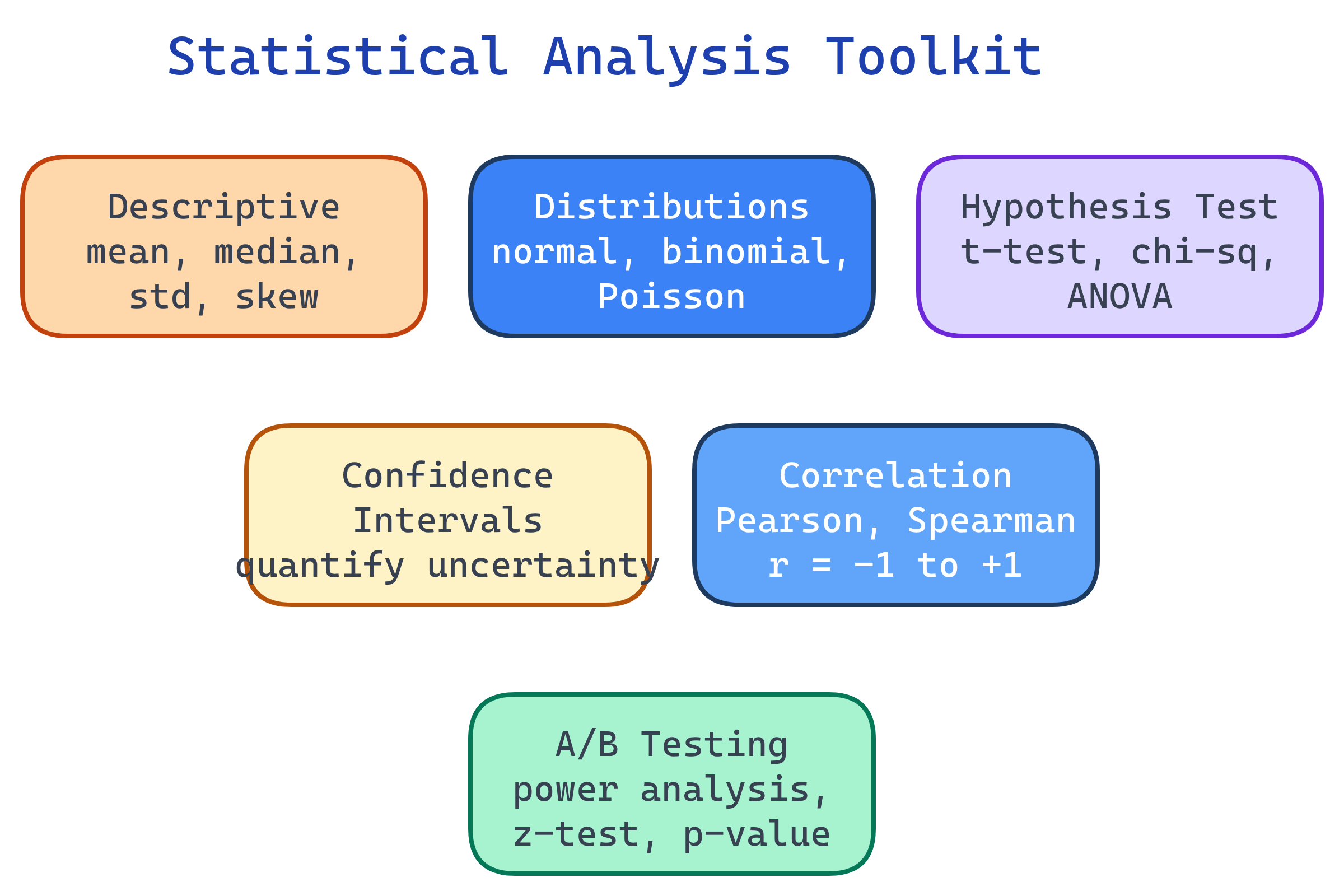
Statistics is the math backbone of data science. Know your distributions (normal, binomial, Poisson), run hypothesis tests (t-test, chi-squared, ANOVA) to prove results aren't random, calculate confidence intervals to quantify uncertainty, and design A/B tests to measure real impact. Python's scipy and statsmodels make it all practical.
Explain Like I'm 12
Imagine you flip a coin 100 times and get 60 heads. Is the coin unfair, or did you just get lucky? Statistics answers that question. It tells you: "There's only a 3% chance of getting 60+ heads with a fair coin, so the coin is probably loaded." That 3% is called a p-value. Statisticians set a threshold (usually 5%) — if the p-value is below it, we say the result is statistically significant (not just luck).
The Statistical Toolkit
Every data science decision involves uncertainty. Statistics gives you tools to quantify that uncertainty and make defensible decisions.
Descriptive Statistics
Before testing hypotheses, summarize your data. These are the numbers that describe the shape and spread of your dataset.
import numpy as np
import pandas as pd

# Central tendency
mean = df['salary'].mean()       # average (sensitive to outliers)
median = df['salary'].median()   # middle value (robust to outliers)
mode = df['salary'].mode()[0]    # most common value

# Spread
std = df['salary'].std()         # standard deviation
var = df['salary'].var()         # variance (std²)
iqr = df['salary'].quantile(0.75) - df['salary'].quantile(0.25)  # IQR

# Shape
skew = df['salary'].skew()      # >0 = right-skewed, <0 = left-skewed
kurt = df['salary'].kurtosis()   # >0 = heavy tails, <0 = light tails

# Quick summary
print(df['salary'].describe())| Measure | What It Tells You | When to Use |
|---|---|---|
| Mean | Average value | Symmetric distributions without outliers |
| Median | Middle value (50th percentile) | Skewed data or data with outliers |
| Standard Deviation | How spread out values are | Understanding variability |
| IQR | Spread of the middle 50% | Robust measure of spread |
| Skewness | Asymmetry direction | Deciding if transforms are needed |
Probability Distributions
A distribution describes the possible values a variable can take and how likely each is. Knowing the right distribution lets you model uncertainty correctly.
Normal (Gaussian) Distribution
The bell curve. Defined by mean (μ) and standard deviation (σ). Most natural phenomena follow it (heights, test scores, measurement errors).
from scipy import stats
import numpy as np

# Generate normally distributed data
data = np.random.normal(loc=100, scale=15, size=1000)  # μ=100, σ=15

# 68-95-99.7 rule
within_1_std = np.mean(np.abs(data - 100) < 15)   # ≈ 68%
within_2_std = np.mean(np.abs(data - 100) < 30)   # ≈ 95%
within_3_std = np.mean(np.abs(data - 100) < 45)   # ≈ 99.7%

# Probability of a value > 130
p = 1 - stats.norm.cdf(130, loc=100, scale=15)  # ≈ 0.023 (2.3%)
print(f"P(X > 130) = {p:.4f}")Other Key Distributions
| Distribution | Use Case | Example |
|---|---|---|
| Binomial | Count of successes in n trials | How many emails are spam out of 100? |
| Poisson | Count of events in a time window | How many support tickets per hour? |
| Exponential | Time between events | Time between customer arrivals |
| Uniform | Equal probability across range | Random number generator output |
| Chi-squared | Sum of squared normal variables | Categorical independence testing |
Hypothesis Testing
Hypothesis testing answers: "Is this result real or just random noise?" You set up two competing hypotheses, collect data, and use a test statistic to decide.
The 5-Step Process
- State hypotheses — H0 (null: no effect) vs Ha (alternative: there is an effect)
- Choose significance level — Usually α = 0.05 (5% chance of false positive)
- Select the right test — Based on data type and question
- Calculate p-value — Probability of seeing this result if H0 is true
- Decide — If p < α, reject H0. If p ≥ α, fail to reject H0
from scipy import stats

# t-test: Is the average salary different from $75,000?
sample_salaries = df['salary'].dropna()
t_stat, p_value = stats.ttest_1samp(sample_salaries, 75000)
print(f"t-statistic: {t_stat:.3f}, p-value: {p_value:.4f}")

if p_value < 0.05:
    print("Reject H0: Average salary IS significantly different from $75K")
else:
    print("Fail to reject H0: No significant difference from $75K")
Choosing the Right Test
| Question | Test | scipy Function |
|---|---|---|
| Is the mean different from a value? | One-sample t-test | stats.ttest_1samp() |
| Are two group means different? | Two-sample t-test | stats.ttest_ind() |
| Are paired measurements different? | Paired t-test | stats.ttest_rel() |
| Are 3+ group means different? | ANOVA | stats.f_oneway() |
| Are two categorical variables related? | Chi-squared test | stats.chi2_contingency() |
| Is the data normally distributed? | Shapiro-Wilk test | stats.shapiro() |
| Non-normal, two groups? | Mann-Whitney U test | stats.mannwhitneyu() |
Confidence Intervals
A confidence interval gives you a range of plausible values for a parameter, not just a single estimate.
from scipy import stats
import numpy as np

sample = df['conversion_rate'].dropna()
mean = sample.mean()
se = stats.sem(sample)  # standard error of the mean

# 95% confidence interval
ci_95 = stats.t.interval(
    confidence=0.95,
    df=len(sample) - 1,
    loc=mean,
    scale=se
)
print(f"Mean: {mean:.4f}")
print(f"95% CI: ({ci_95[0]:.4f}, {ci_95[1]:.4f})")
# "We're 95% confident the true conversion rate is between X and Y"Correlation
Correlation measures the strength and direction of a linear relationship between two variables. It ranges from -1 (perfect negative) to +1 (perfect positive).
import pandas as pd

# Pearson correlation (linear relationships, assumes normality)
pearson_corr = df['study_hours'].corr(df['exam_score'])

# Spearman correlation (monotonic relationships, robust to outliers)
spearman_corr = df['study_hours'].corr(df['exam_score'], method='spearman')

# Full correlation matrix
corr_matrix = df.select_dtypes(include='number').corr()

# Statistical significance of correlation
from scipy import stats
r, p_value = stats.pearsonr(df['study_hours'], df['exam_score'])
print(f"r = {r:.3f}, p = {p_value:.4f}")A/B Testing
A/B testing is hypothesis testing applied to real-world experiments. Show group A the current version, group B the new version, and measure if B is better.
from scipy import stats
import numpy as np

# Example: Testing a new checkout button
# Group A (control): 1000 users, 50 conversions (5.0%)
# Group B (variant): 1000 users, 65 conversions (6.5%)

n_a, conv_a = 1000, 50
n_b, conv_b = 1000, 65

rate_a = conv_a / n_a  # 0.050
rate_b = conv_b / n_b  # 0.065

# Two-proportion z-test
from statsmodels.stats.proportion import proportions_ztest

count = np.array([conv_b, conv_a])
nobs = np.array([n_b, n_a])

z_stat, p_value = proportions_ztest(count, nobs, alternative='larger')
print(f"Z-statistic: {z_stat:.3f}")
print(f"P-value: {p_value:.4f}")

# Effect size (relative lift)
lift = (rate_b - rate_a) / rate_a * 100
print(f"Lift: {lift:.1f}%")

# Sample size calculator (for planning)
from statsmodels.stats.power import NormalIndPower
analysis = NormalIndPower()
sample_size = analysis.solve_power(
    effect_size=0.1,  # expected small effect
    alpha=0.05,
    power=0.8,        # 80% chance of detecting the effect
    ratio=1            # equal group sizes
)
print(f"Required sample per group: {int(np.ceil(sample_size))}")Test Yourself
Your A/B test shows a p-value of 0.03. The conversion rate improved from 4.0% to 4.2%. Should you ship the change?
What's the difference between a Type I and Type II error?
When would you use Spearman correlation instead of Pearson?
You have 3 groups and want to compare their means. Why can't you just run 3 t-tests?
What does a 95% confidence interval actually mean?
Interview Questions
Explain the Central Limit Theorem and why it matters for data science.
Your A/B test has been running for a week and the p-value is 0.06. Should you run it longer?
How would you handle multiple comparisons in a hypothesis testing scenario?