Machine Learning Fundamentals
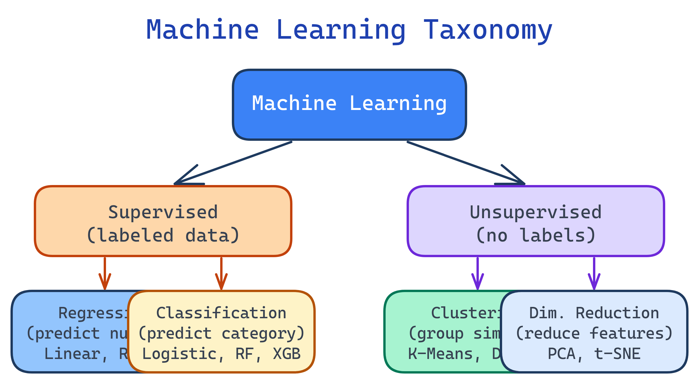
Machine learning teaches computers to learn from data. Supervised learning uses labeled data (regression for numbers, classification for categories). Unsupervised learning finds patterns without labels (clustering, dimensionality reduction). Key algorithms: Linear Regression, Logistic Regression, Decision Trees, Random Forest, XGBoost, K-Means. Always split data, tune hyperparameters, and watch for overfitting.
Explain Like I'm 12
Imagine you're learning to recognize dogs vs cats. Supervised learning is like having a teacher show you labeled photos: "This is a dog, this is a cat." After enough examples, you can label new photos yourself. Unsupervised learning is like sorting a pile of photos into groups without being told what's what — you notice some have pointy ears and some have round ears. Overfitting is like memorizing the exact photos instead of learning the general idea — you'd fail on new photos you haven't seen.
The ML Landscape
Machine learning algorithms fall into three main categories based on how they learn from data.
Supervised Learning
You give the algorithm inputs (features) and correct answers (labels). It learns the mapping from inputs to outputs, then predicts labels for new data.
Regression (Predicting Numbers)
When your target is a continuous number — house prices, temperature, revenue.
from sklearn.linear_model import LinearRegression
from sklearn.model_selection import train_test_split
from sklearn.metrics import mean_squared_error, r2_score
import numpy as np

X_train, X_test, y_train, y_test = train_test_split(
    X, y, test_size=0.2, random_state=42
)

# Linear Regression: simplest baseline
model = LinearRegression()
model.fit(X_train, y_train)
y_pred = model.predict(X_test)

print(f"RMSE: {np.sqrt(mean_squared_error(y_test, y_pred)):.2f}")
print(f"R² Score: {r2_score(y_test, y_pred):.3f}")

# Feature importance (coefficients)
for feat, coef in zip(X.columns, model.coef_):
print(f" {feat}: {coef:.3f}")Classification (Predicting Categories)
When your target is a category — spam/not spam, churn/retain, disease/healthy.
from sklearn.linear_model import LogisticRegression
from sklearn.metrics import classification_report, confusion_matrix

model = LogisticRegression(max_iter=1000)
model.fit(X_train, y_train)
y_pred = model.predict(X_test)

# Confusion matrix: actual vs predicted
print(confusion_matrix(y_test, y_pred))
# [[TN, FP],
#  [FN, TP]]

# Full report
print(classification_report(y_test, y_pred))| Algorithm | Type | Best For | Pros | Cons |
|---|---|---|---|---|
| Linear Regression | Regression | Linear relationships | Fast, interpretable | Assumes linearity |
| Logistic Regression | Classification | Binary outcomes | Fast, probabilistic | Linear decision boundary |
| Decision Tree | Both | Non-linear, interpretable | Easy to visualize | Overfits easily |
| Random Forest | Both | General purpose | Robust, feature importance | Slow on large data |
| XGBoost | Both | Tabular data competitions | Best accuracy often | More hyperparameters |
| KNN | Both | Small datasets | Simple, no training | Slow at prediction time |
Unsupervised Learning
No labels — the algorithm discovers structure in the data on its own. Used for customer segmentation, anomaly detection, and dimensionality reduction.
Clustering (Grouping Similar Items)
from sklearn.cluster import KMeans
from sklearn.preprocessing import StandardScaler

# Always scale features before clustering
scaler = StandardScaler()
X_scaled = scaler.fit_transform(X)

# K-Means: group customers into 4 segments
kmeans = KMeans(n_clusters=4, random_state=42, n_init=10)
df['cluster'] = kmeans.fit_predict(X_scaled)

# Analyze clusters
print(df.groupby('cluster')[['age', 'income', 'spending']].mean())

# How to pick K? Elbow method
inertias = []
for k in range(1, 11):
    km = KMeans(n_clusters=k, random_state=42, n_init=10)
    km.fit(X_scaled)
inertias.append(km.inertia_)StandardScaler puts all features on the same scale.Dimensionality Reduction
Reduce the number of features while preserving the most important information. PCA (Principal Component Analysis) is the most common method.
from sklearn.decomposition import PCA
import matplotlib.pyplot as plt

# Reduce 50 features down to 2 for visualization
pca = PCA(n_components=2)
X_2d = pca.fit_transform(X_scaled)

# How much variance does each component explain?
print(f"Explained variance: {pca.explained_variance_ratio_}")
# e.g., [0.45, 0.20] = first 2 components capture 65% of variance

# Plot
plt.scatter(X_2d[:, 0], X_2d[:, 1], c=df['cluster'], cmap='viridis')
plt.xlabel('PC1')
plt.ylabel('PC2')
plt.title('Customer Segments (PCA)')
plt.show()The Bias-Variance Tradeoff
The fundamental challenge in ML: your model must be complex enough to capture real patterns (low bias) but simple enough to generalize to new data (low variance).
| Underfitting (High Bias) | Good Fit | Overfitting (High Variance) | |
|---|---|---|---|
| Train Score | Low | High | Very High (~100%) |
| Test Score | Low | High (close to train) | Low (big gap from train) |
| Model | Too simple | Just right | Too complex |
| Fix | More features, complex model | Ship it! | More data, regularization, simpler model |
# Detect overfitting: compare train vs test scores
from sklearn.ensemble import RandomForestClassifier

model = RandomForestClassifier(n_estimators=100, random_state=42)
model.fit(X_train, y_train)

train_score = model.score(X_train, y_train)
test_score = model.score(X_test, y_test)

print(f"Train: {train_score:.3f}")
print(f"Test:  {test_score:.3f}")
# If train ≈ 0.99 and test ≈ 0.75 → overfitting!

# Fix: reduce complexity
model = RandomForestClassifier(
    n_estimators=100,
    max_depth=10,        # limit tree depth
    min_samples_leaf=5,  # require more samples per leaf
    random_state=42
)Hyperparameter Tuning
Hyperparameters are settings you choose before training (like max_depth, n_estimators). Use grid search or random search to find the best combination.
from sklearn.model_selection import GridSearchCV

param_grid = {
    'n_estimators': [100, 200, 500],
    'max_depth': [5, 10, 20, None],
    'min_samples_leaf': [1, 2, 5]
}

grid = GridSearchCV(
    RandomForestClassifier(random_state=42),
    param_grid,
    cv=5,
    scoring='f1',
    n_jobs=-1  # use all CPU cores
)
grid.fit(X_train, y_train)

print(f"Best params: {grid.best_params_}")
print(f"Best CV F1:  {grid.best_score_:.3f}")

# Use the best model
best_model = grid.best_estimator_
print(f"Test F1: {best_model.score(X_test, y_test):.3f}")RandomizedSearchCV instead of GridSearchCV when you have many hyperparameters. It samples random combinations and is much faster while finding nearly-as-good results.Test Yourself
You're predicting whether a customer will churn (yes/no). Which type of ML problem is this, and what's a good baseline algorithm?
Your model has 98% training accuracy but 72% test accuracy. What's happening and how do you fix it?
max_depth, increase min_samples_leaf). 3) Add regularization (L1/L2). 4) Remove noisy or redundant features. 5) Use cross-validation instead of a single split.Why do you need to scale features before K-Means clustering?
StandardScaler) puts all features on the same scale so each contributes equally to the distance calculation.When would you use PCA?
What's the difference between GridSearchCV and RandomizedSearchCV?
Interview Questions
Explain the bias-variance tradeoff. How does it relate to model complexity?
How does Random Forest improve on a single Decision Tree?
When would you choose Logistic Regression over Random Forest?
What is regularization and why is it used?