ML Model Lifecycle
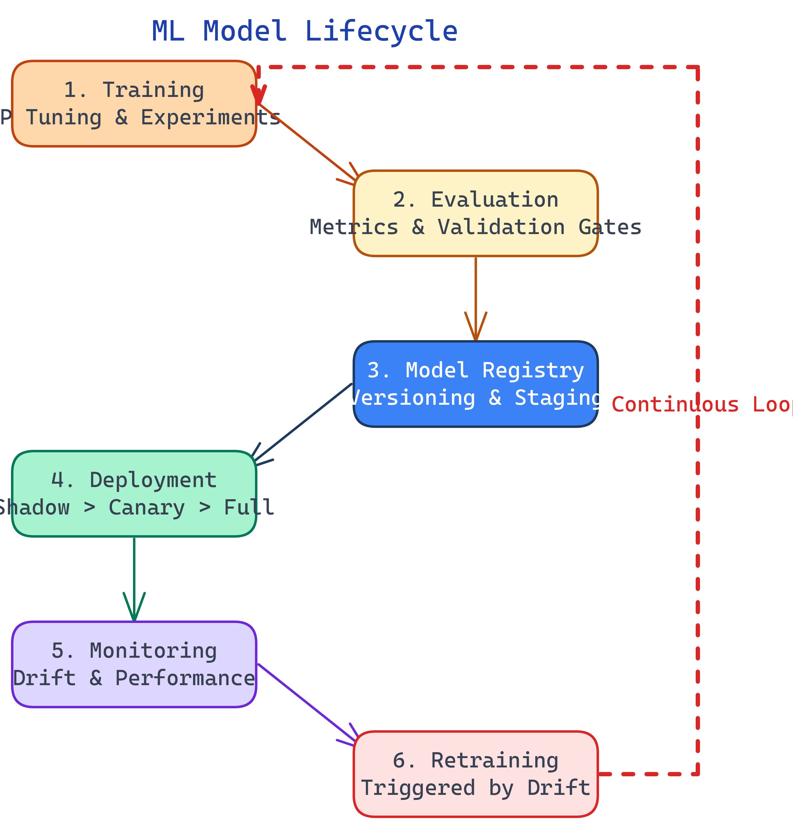
An ML model's journey: train (experiments, hyperparameter tuning), evaluate (offline metrics, validation sets), register (version in model registry), deploy (shadow mode, canary, blue-green), monitor (data drift, prediction drift, latency), and retrain (triggered by drift or on a schedule). The lifecycle never ends — it loops.
The Big Picture
Explain Like I'm 12
Think of a weather forecasting robot. You train it by showing it years of weather data. Then you test it: did it correctly predict rain on days it actually rained? If it scores well, you publish the forecast to the newspaper. Every day you check: is it still getting the forecasts right? If it starts predicting snow in July, you retrain it with newer data. Train → test → publish → watch → retrain. Over and over.
Training
Training is where you teach the model to find patterns in data. In production MLOps, training is not a one-off notebook — it's an automated, reproducible pipeline.
Hyperparameter Tuning
Models have knobs you set before training: learning rate, number of layers, batch size, regularization strength. Finding the best combination is hyperparameter tuning.
| Strategy | How It Works | When to Use |
|---|---|---|
| Grid Search | Try every combination from a predefined grid | Small search space, few parameters |
| Random Search | Sample random combinations | Large search space, faster than grid |
| Bayesian Optimization | Use previous results to guide the next trial | Expensive training runs (deep learning) |
import optuna

def objective(trial):
    lr = trial.suggest_float("lr", 1e-5, 1e-1, log=True)
    n_layers = trial.suggest_int("n_layers", 1, 5)
    dropout = trial.suggest_float("dropout", 0.1, 0.5)

    model = build_model(lr=lr, n_layers=n_layers, dropout=dropout)
    accuracy = train_and_evaluate(model, X_train, y_train, X_val, y_val)
    return accuracy

study = optuna.create_study(direction="maximize")
study.optimize(objective, n_trials=100)

print(f"Best params: {study.best_params}")
print(f"Best accuracy: {study.best_value:.4f}")Evaluation
Before a model goes to production, it must pass offline evaluation. This means measuring it against a held-out test set that the model has never seen.
Key metrics depend on the task:
| Task | Metrics | Watch out for |
|---|---|---|
| Classification | Accuracy, Precision, Recall, F1, AUC-ROC | Class imbalance — 99% accuracy is meaningless if 99% of data is one class |
| Regression | MAE, RMSE, R² | Outliers can skew RMSE — check MAE too |
| Ranking | NDCG, MAP, MRR | Position bias — users click top results regardless of quality |
Model Validation Gates
Automated validation gates prevent bad models from reaching production. Your pipeline should check:
- Metrics exceed minimum thresholds (e.g., F1 > 0.85)
- New model outperforms the current production model (champion/challenger)
- No data leakage detected
- Inference latency is within SLA (e.g., p99 < 100ms)
- Bias/fairness checks pass for protected attributes
Deployment Strategies
Deploying a model is riskier than deploying code because a bad model produces wrong answers, not error pages. Use progressive rollout strategies:
Shadow Mode
The new model runs alongside the current one but its predictions are logged, not served to users. You compare both models' predictions on real traffic without any risk. This is the safest first step for high-stakes models (financial, medical).
Canary Deployment
Route a small percentage of traffic (e.g., 5%) to the new model. Monitor metrics. If healthy, gradually increase (10%, 25%, 50%, 100%). If metrics degrade, roll back immediately — only 5% of users were affected.
Blue-Green Deployment
Run two identical environments. Blue serves the current model. Green gets the new model. Switch traffic all at once after testing. Instant rollback by switching back to Blue.
A/B Testing
Split traffic between the old model (control) and new model (treatment). Measure a business metric (revenue, conversion, engagement), not just ML metrics. Run until statistically significant. This is the gold standard for validating that a better model actually improves the product.
Monitoring in Production
Models don't crash — they silently degrade. That makes monitoring critical. Here's what to watch:
Data Drift Detection
Compare the distribution of incoming features against the training data. Statistical tests like Kolmogorov-Smirnov (for numerical features) and chi-squared (for categorical features) can detect when distributions diverge.
from evidently.test_suite import TestSuite
from evidently.tests import TestColumnDrift

# Test for drift on key features
suite = TestSuite(tests=[
    TestColumnDrift(column_name="transaction_amount"),
    TestColumnDrift(column_name="user_age"),
    TestColumnDrift(column_name="device_type"),
])
suite.run(reference_data=train_df, current_data=prod_df)

# Check if any test failed
if not suite.as_dict()["summary"]["all_passed"]:
    trigger_retraining_pipeline()
Performance Monitoring
When ground truth arrives (which can be delayed by hours, days, or weeks), compute actual accuracy. Set up dashboards tracking:
- Accuracy / F1 / AUC over time (rolling windows)
- Prediction distribution (are predictions shifting?)
- Feature importance stability
- Latency (p50, p95, p99)
- Throughput (requests per second)
Retraining Strategies
When should you retrain? There are three triggers:
- Scheduled retraining — Retrain on a fixed cadence (daily, weekly, monthly). Simple and predictable. Use when data arrives regularly.
- Drift-triggered retraining — Retrain when monitoring detects significant data or prediction drift. More efficient — you only retrain when needed.
- Performance-triggered retraining — Retrain when actual metrics drop below a threshold. Most accurate trigger, but requires ground truth labels.
Test Yourself
What is shadow mode deployment and when should you use it?
Why are offline metrics (test set accuracy) not sufficient for production?
Explain the champion/challenger pattern.
What's the difference between data drift and concept drift?
Name three triggers for model retraining.
Interview Questions
Q: How would you deploy a new ML model to production with minimal risk?
Q: Your model accuracy dropped 10% overnight. Walk me through your debugging process.
Q: How do you handle ground truth delay when monitoring model performance?